DAY 2 Ohm Law - KCL - KVL /Resistors and Ohms Law - Voltage-Current Characteristics/Dependent Sources and MOSFETs

Today we learn about Ohm Law - KCL - KVL. As normal, we begin the class with a question from the professor. And here is our answer. If the supplies have the same voltage, the bulbs stay the same as the result of the equations. However, if the supplies have different voltages. the bulbs will change.

After that, we study about Ohm Law with state that Ohm’s law states that the voltage v across a resistor is directly proportional to the current i flowing through the resistor. We practice with the problem about the "hot" resistance and "cold" resistance. For the "hot" resistance we apply Ohm Law, while the "cold" we need use our "educated guessing" to find the answer which should be smaller than the "hold" resistance. 

The Lab About Resistors and Ohms Law - Voltage-Current Characteristics
Purpose:

The lab aims to help us get the practical verification of Ohm Law relating to the voltage and current characteristics, as well as studying some basic knowledge about statistic to apply for graphing or ploting. 
Procedure:

We set up the devices as the picture below to measure the current of the circuit that has the variable voltage, the waveform generator.


Tips:
The power of the waveform generator is always off, so need to turn it on before operating.
The direct voltage is used in this lab.
The cable of the waveform need to connect correctly as the instruction
 
In this lab, we use the yellow cable for the waveform generator and the black cable for the ground connection.

Results:
1. The resistance of the resistor, directly measured by the Ohmmeter and subtracted the resistance of the wire, is 100.6 Ohm.
2. The table providing ir from vs

3. The table for the vr, which measured separately in another set-up, and ir. And the equation for least-squares best fist line to the data and the correlation coefficient between the data and the curve fit.

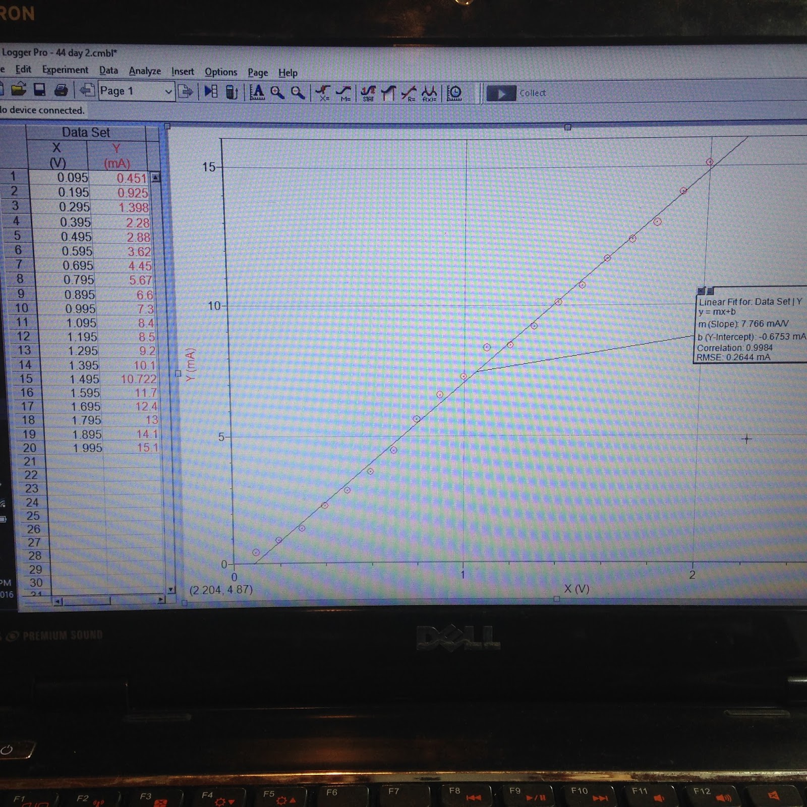
The correlation is 0.9984 or 99.84%, then the data almost fit the linear relationship.
I have the equation is i=7.666(mA/V).v => R=v/i=130 Ohm.

Nodes, Branches And Loops

In the next course time, we study about the nodes, branches, and loops. We study the definition of the three physical terms and learn how to classify them in a circuit. 

We learn about the formula Branches = Loops + Nodes -1. We do one practice problem and find out that the L in the formula stands for the independent loops, not every single loop we find in the circuit. 

Kirchhoff’s LAWS

The important part of today is about Kirchoff's LAWS. This law includes two small laws: one for current KCL, and one for voltage KVL.

The practice for this section is below

We have to choose reasonable and logical direction of the voltage for this problem to work it throughout.

Dependent Sources and MOSFETs
Purpose:
This lab gives us the fundamental view about MOSFET properties.

Procedure:
Follow this diagram,

Set up the circuit as the picture below

The analog now takes two roles in this lab. It creates a 5V source and a changeable voltage/waveform generator. For the waveform generator, we connect the yellow cable (W1 standing for channel 1) to the gate G of the MOSFET. For the 5V source, we connect the  red cable to the drain D. Meanwhile, the two ground cable of the analog are connected to the source of the MOSFET.

Results:
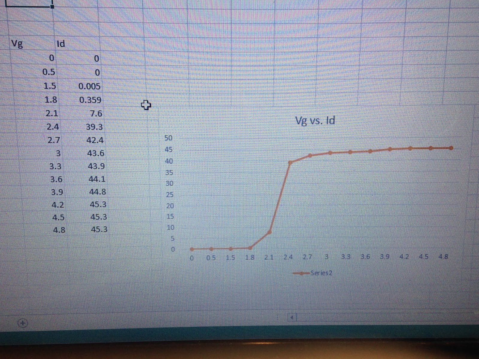
In the picture is the table providing our measured gate-to-source voltage vs. drain current values



1.The measured resistance value is 100.6 Ohm.
2. MOSFET threashold voltage is 0.005mA.
3. The transistor or MOSFET behaves as a nonlinear dependent source. Because it need the threashold voltage to create current passing the MOSFET, and when the voltage is equal to 4.5 and higher, the value of the current is unchanged.
We try to fit a straight line to the data which have the changes between the voltage and the current. We acquire the equation below with the slope of the line is 18.51(mA/V), and the correlation is 0.85.

In summary, this class we learn about Ohm Law and Kirchhoff's Law Besides, we operate one lab in order to expand our understanding of Ohm Law, and we also perform another lab about a transistor MOSFET to learn about its basic characteristic.

DAY 1: MATLAB

INTRODUCTION TO NUMERICAL COMPUTATION

USING MATLAB AS A CALCULATOR

6+3/2

ans =

    7.5000

>> 3+4

ans =

     7

>> (6+3)/2

ans =

    4.5000

>> 11^2

ans =

   121

>> 2*3+4^3

ans =

70

MATH FUNCTIONS

3=4

 3=4

  |Error: The expression to the left of the equals sign is not a valid target for an assignment.

 >> 3+4

ans =

     7

ASSIGNING EXPRESSIONS TO VARIABLES

x=2*5

x =

    10

>> x

x =

    10

>> x=2*5;

>> x

x =

    10

CREATING AN ARRAY

            CREATING A ROW VECTOR

>> X= [2 4 5 6 7]

X =

     2     4     5     6     7

            CREATING A COLUMN VECTOR

Y=[3;5;3;5;6]

Y =

     3

     5

     3

     5

     6

            CREATING A MATRIX

XY=[1 1 1 1;2 2 2 2;3 3]

Error using vertcat

Dimensions of matrices being concatenated are not consistent.

 >> XY=[1 1 1 1;2 2 2 2;3 3 3 3]

XY =

     1     1     1     1

     2     2     2     2

     3     3     3     3

1.        C=[1 2 3;4 5 6;7 8 9]

C =

     1     2     3

     4     5     6

     7     8     9

AUTOMATICALLY CREATING VECTORS

Using the Colon

R=0:0.5:10

R =

  Columns 1 through 11

         0    0.5000    1.0000    1.5000    2.0000    2.5000    3.0000    3.5000    4.0000    4.5000    5.0000

  Columns 12 through 21

    5.5000    6.0000    6.5000    7.0000    7.5000    8.0000    8.5000    9.0000    9.5000   10.0000

TRANSPOSING ARRAYS

test1=[2 3 4 5]

test1 =

     2     3     4     5

>> tes2=test1'

tes2 =

     2

     3

     4

     5

>> xx=[1 1;2 2;3 3]

xx =

     1     1

     2     2

     3     3

>> xx=xx'

xx =

     1     2     3

     1     2     3

APPLYING FUNCTIONS TO ROW VECTORS

x=[0:pi/10:2*pi]

x =

  Columns 1 through 11

         0    0.3142    0.6283    0.9425    1.2566    1.5708    1.8850    2.1991    2.5133    2.8274    3.1416

  Columns 12 through 21

    3.4558    3.7699    4.0841    4.3982    4.7124    5.0265    5.3407    5.6549    5.9690    6.2832

y =

  Columns 1 through 11

         0    0.3090    0.5878    0.8090    0.9511    1.0000    0.9511    0.8090    0.5878    0.3090    0.0000

  Columns 12 through 21

   -0.3090   -0.5878   -0.8090   -0.9511   -1.0000   -0.9511   -0.8090   -0.5878   -0.3090   -0.0000

>> z=cos(x)

The results make sense.

z =

  Columns 1 through 11

    1.0000    0.9511    0.8090    0.5878    0.3090    0.0000   -0.3090   -0.5878   -0.8090   -0.9511   -1.0000

  Columns 12 through 21

   -0.9511   -0.8090   -0.5878   -0.3090   -0.0000    0.3090    0.5878    0.8090    0.9511    1.0000

>> g=exp(x)

g =

  Columns 1 through 11

    1.0000    1.3691    1.8745    2.5663    3.5136    4.8105    6.5861    9.0170   12.3453   16.9020   23.1407

  Columns 12 through 21

   31.6821   43.3762   59.3867   81.3068  111.3178  152.4060  208.6603  285.6784  391.1245  535.4917

>> h=log10(x)

h =

  Columns 1 through 11

      -Inf   -0.5029   -0.2018   -0.0257    0.0992    0.1961    0.2753    0.3422    0.4002    0.4514    0.4971

  Columns 12 through 21

    0.5385    0.5763    0.6111    0.6433    0.6732    0.7013    0.7276    0.7524    0.7759    0.7982

ARRAY OPERATIONS

BB=cos(x)-sin(x)

BB =

  Columns 1 through 11

    1.0000    0.6420    0.2212   -0.2212   -0.6420   -1.0000   -1.2601   -1.3968   -1.3968   -1.2601   -1.0000

  Columns 12 through 21

   -0.6420   -0.2212    0.2212    0.6420    1.0000    1.2601    1.3968    1.3968    1.2601    1.0000

=> MAKE SENSE

>> CC=cos(x)*sin(x)

Error using  *

Inner matrix dimensions must agree.

 >> DD=cos(x).*sin(x)

DD =

  Columns 1 through 11

         0    0.2939    0.4755    0.4755    0.2939    0.0000   -0.2939   -0.4755   -0.4755   -0.2939   -0.0000

  Columns 12 through 21

    0.2939    0.4755    0.4755    0.2939    0.0000   -0.2939   -0.4755   -0.4755   -0.2939   -0.0000

=> MAKE SENSE

ADDRESSING ARRAYS

            ADDRESSING SINGLE DIMENSIONAL ARRAYS

            ADDRESSING MATRICES

>> xy=[1 2 3;4 5 6;7 8 9]

xy =

     1     2     3

     4     5     6

     7     8     9

>> xy(1,1)

ans =

     1

>> xy(1,:)

ans =

     1     2     3

>> xy(:,1)

ans =

     1

     4

     7

>> xy(1:2,:)

ans =

     1     2     3

     4     5     6

>> xy(:,2:3)

ans =

     2     3

     5     6

     8     9

CREATING SIMPLE PLOTS

CREATIG A 2-D PLOT WITHOUT STYLE OPTIONS

degree=0:2*pi/100:2*pi;

>> output=sin(degree);

>> plot(degree,output)

                                   ADDING ADDITIONAL PLOTS TO THE SAME GRAPHS

degree=0:2*pi/100:2*pi;

>> output=sin(degree);

>> plot(degree,output)

>> hold off

>> degree=0:2*pi/100:2*pi;

>> output=sin(degree);

>> plot(degree,output)

>> hold on

>> degree1=0:2*pi/100:2*pi;

>> output1=cos(degree);

>> plot(degree1,output1)

hold off

>> degree=0:2*pi/100:2*pi;

>> output=sin(degree);

>> plot(degree,output)

Plot(degree,sin(degree),degree,cos(degree))

SCRIPT FILES

As to run script need to address the script location to matllab, or save it to matlab.

script

%test script square

square=a^2;

squareroot=sqrt(a);

command window

>> a=4;

>> mt;

>> square

square =

    16

>> squareroot

squareroot =

     2

SOLVING SIMULTANEOUS EQUATIONS

ASSIGNMENT 1:

>> r=[1 -1 -1;20 0 10;0 5 -10]

r =

     1    -1    -1

    20     0    10

     0     5   -10

>> v=[0;15;7]

v =

     0

    15

     7

>> i=inv(r)*v

i =

    0.8429

    1.0286

   -0.1857

=> R3= -0.1857

PLOTING EXPONETIALS

>> plot(t,x1,t,x2,t,x3)

>> tau1=1;

>> tau2=tau1*0.5;

>> tau3=tau1*2;

>> x1=5*exp(-t/tau1);

>> x2=5*exp(-t/tau2);

>> x3=5*exp(-t/tau3);

>> plot(t,x1,t,x2,t,x3)

 

ADDING SINUSOIDS

ASSIGNMENT 1

1. >> t=linspace(0,500);

>> ca=2*(exp(-t/100));

>> cb=2*(exp(-t/200));

>> plot(t,ca)

>> plot(t,cb)

>> plot(t,ca,t,cb)

ca will have the lowest output sooner.

>> ca2=2*(1-exp(-t/100));

>> cb2=2*(1-exp(-t/200));

>> plot(t,ca2,t,cb2)

>> plot(t,ca2)

>> plot(t,cb2)

2, Assignment 2

t=linspace(0,4*pi);

>> theo=7.29*sin(2*t+0.727);

>> mat=3*sin(2*t+10*pi/180)+5*cos(2*t-30*pi/180);

>> plot(t,theo,t,mat);

>> mat1=3*sin(2*t+10*pi/180);

>> mat2=5*cos(2*t-30*pi/180);

>> plot(t,theo,t,mat,t,mat1,t,mat2)

2.

f=10;

>> w=2*pi*f;

>> theo=7.29*sin(w*t+0.727);

>> mat=3*sin(w*t+10*pi/180)+5*cos(w*t-30*pi/180);

>> plot(t,theo,t,mat);

A Script to implement this with any f(HZ)

>> w=2*pi*f;

>> theo=7.29*sin(w*t+0.727);

>> mat=3*sin(w*t+10*pi/180)+5*cos(w*t-30*pi/180);

>> plot(t,theo,t,mat);

f=20;

>> assi

COMPLEX NUMBER

OPERATIONS WITH COMPLEX NUMBERS

>> A=2+2j, B=-1+3j, C=2+j

A =

   2.0000 + 2.0000i

B =

  -1.0000 + 3.0000i

C =

   2.0000 + 1.0000i

>> D=(A*B)/C

D =

  -2.4000 + 3.2000i

>> E=(A+B)*C

E =

  -3.0000 +11.0000i

FUNCTIONS TO CONVERT FROM RECTANGULAR TO POLAR

EXERCISE 1:

>> A=3+4j; B=3-2j; C=2*exp(50*pi/180*j);

>> D=(A+C)/B

D =

   0.1379 + 1.9360i

EXERCISE 2:

>> E

E =

  -3.0000 +11.0000i

>> abs(E)

ans =

   11.4018

>> angle(E)

ans =

    1.8370

>> angle(E)*180/pi

ans =

  105.2551

ASSIGNMENT

>> A1=3+2j; A2=-1+4j; B=2-2j

B =

   2.0000 - 2.0000i

>> A1=3+2j; A2=-1+4j; B=2-2j;

>> C=(A1*B)/A2

C =

  -1.0588 - 2.2353i

2.

>> angle(A1)*180/pi, abs(A1)

ans =

   33.6901

ans =

    3.6056

>> %3.6056<33.6901

>> angle(A2)*180/pi, abs(A2)

ans =

  104.0362

ans =

    4.1231

>>%4.1<104

>> 4<104

ans =

     1

>> angle(B)*180/pi, abs(B)

ans =

   -45

ans =

    2.8284

>> %2.8<-45

3.

>> D=(A1+B)*A2

D =

  -5.0000 +20.0000i

4.

>> T=[8+8j 2j;2j 4-4j]

>> P=[50j;-30j]

>> I=inv(T)*P

I =

   2.0588 + 2.9412i

   5.0000 - 3.5294i

>> I2=5-3.5294j; angle(I2)*180/pi, abs(I2)

ans =

  -35.2175

ans =

    6.1202

SOLVING FOR ROOTS OF EQUATIONS

EXERCISE 1

>> p=[1 4 3];

>> r=roots(p)

r =

    -3

-1

Assignment

1. >> p1=[1 1 4];

>> p2=[1 3 0 3];

>> p3=[1 3 4 2 7];

>> r1=roots(p1)

r1 =

  -0.5000 + 1.9365i

  -0.5000 - 1.9365i

>> r2=roots(p2)

r2 =

  -3.2790 + 0.0000i

   0.1395 + 0.9463i

   0.1395 - 0.9463i

>> r3=roots(p3)

r3 =

  -1.8222 + 1.2680i

  -1.8222 - 1.2680i

   0.3222 + 1.1474i

   0.3222 - 1.1474i

2.
>> p=[1 5 7 3];
>> s=roots(p)
s =
  -3.0000 + 0.0000i
  -1.0000 + 0.0000i
  -1.0000 - 0.0000i

>>  T=[1 1 0;2 4 1;1 3 3];
>> I=[0;1;7];
>> K=inv(T)*I

K =

     1
    -1
     3

DAY 1: Current and Voltage/ Solderless Breadboard, Open-circuits and Shot-circuits

Current and Voltage 

The first question of the semester, what will happen when the switch is on? The answer is the bulbs stay the same because there is no different voltage between the wire of the switch, or the current does not pass through this wire.

the problem for the current definition: the time rate of change of charge. We find the function of charge in term of time and derivative it to get the current in term of time. 

Problem for the power and energy. From the graph i vs. t, we get the graph W vs. t and p vs.t through these formula p=v.i, and p=dw/dt => w= integral(p.dt)

From v vs.t and i vs. t graph, we get the p vs. t and w vs.t graph. we interpret the graph into the equation i(t) and v(t), then apply these formula to get the answer p=vi and w=integral(p.dt).

By applied the theory that the sum of the power in all elements is 0, we get the answer for the above problem

Lab: Solderless Breadboard, Open-circuits and Shot-circuits

Purpose:

This lab aims to give students the fundamental understanding of a breadboard where is the open-circuit and where is the short-circuit.

Procedure:

We use wires and digital multimeter as an Ohmmeter to check resistance in order to verify the circuits of a breadboard.  

1. Firstly, we measure the resistance between two holes in the same row. The DMM reads 0.4 Ohm , so it is a short-circuit. 

 

2. Secondly, we measure the resistance between two holes on opposite sides of the central channel of the breadboard. The DMM reads infinite Ohm , so it is an open-circuit.

 

3. Thirdly, we measure between two arbitrary holes in the breadboard. The DMM reads infinite Ohm, so it is an open-circuit.

 

4. Lastly, we measure between holes connected by a jumper wire. The DMM reads 3 Ohm, so it is a short-circuit.

We have the results in the white board. 1 and 4 are the short-circuits, while 2 and 3 are the open-circuits.

In conclusion

We learn about the basic property of the breadboard through this lab. We distinguish between the short circuit and open circuit. As the results showing, the connection inside a breadboard is the same like the following picture.