USING MATLAB AS A
CALCULATOR
6+3/2
ans =
7.5000
>> 3+4
ans =
7
>> (6+3)/2
ans =
4.5000
>> 11^2
ans =
121
>> 2*3+4^3
ans =
70
MATH FUNCTIONS
3=4
3=4
|Error: The expression to the left of the equals sign is not a valid
target for an assignment.
>> 3+4
ans =
7
ASSIGNING EXPRESSIONS TO VARIABLES
x=2*5
x =
10
>> x
x =
10
>> x=2*5;
>> x
x =
10
CREATING AN ARRAY
CREATING A ROW VECTOR
>> X= [2 4 5 6 7]
X =
2
4 5 6
7
CREATING A COLUMN
VECTOR
Y=[3;5;3;5;6]
Y =
3
5
3
5
6
CREATING A MATRIX
XY=[1 1 1 1;2 2 2 2;3 3]
Error using vertcat
Dimensions of matrices being
concatenated are not consistent.
>> XY=[1 1 1 1;2 2 2 2;3 3 3 3]
XY =
1
1 1 1
2
2 2 2
3
3 3 3
1. C=[1 2 3;4 5 6;7 8 9]
C =
1
2 3
4
5 6
7
8 9
AUTOMATICALLY CREATING VECTORS
Using the Colon
R=0:0.5:10
R =
Columns 1 through 11
0
0.5000 1.0000 1.5000
2.0000 2.5000 3.0000
3.5000 4.0000 4.5000
5.0000
Columns 12 through 21
5.5000
6.0000 6.5000 7.0000
7.5000 8.0000 8.5000
9.0000 9.5000 10.0000
TRANSPOSING ARRAYS
test1=[2 3 4 5]
test1 =
2
3 4 5
>> tes2=test1'
tes2 =
2
3
4
5
>> xx=[1 1;2 2;3 3]
xx =
1
1
2
2
3
3
>> xx=xx'
xx =
1
2 3
1
2 3
APPLYING FUNCTIONS TO ROW VECTORS
x=[0:pi/10:2*pi]
x =
Columns 1 through 11
0
0.3142 0.6283 0.9425
1.2566 1.5708 1.8850
2.1991 2.5133 2.8274
3.1416
Columns 12 through 21
3.4558
3.7699 4.0841 4.3982
4.7124 5.0265 5.3407
5.6549 5.9690 6.2832
y =
Columns 1 through 11
0
0.3090 0.5878 0.8090
0.9511 1.0000 0.9511
0.8090 0.5878 0.3090
0.0000
Columns 12 through 21
-0.3090 -0.5878 -0.8090
-0.9511 -1.0000 -0.9511
-0.8090 -0.5878 -0.3090
-0.0000
>> z=cos(x)
The results make sense.
z =
Columns 1 through 11
1.0000
0.9511 0.8090 0.5878
0.3090 0.0000 -0.3090
-0.5878 -0.8090 -0.9511
-1.0000
Columns 12 through 21
-0.9511 -0.8090 -0.5878
-0.3090 -0.0000 0.3090
0.5878 0.8090 0.9511
1.0000
>> g=exp(x)
g =
Columns 1 through 11
1.0000
1.3691 1.8745 2.5663
3.5136 4.8105 6.5861
9.0170 12.3453 16.9020
23.1407
Columns 12 through 21
31.6821 43.3762 59.3867
81.3068 111.3178 152.4060
208.6603 285.6784 391.1245
535.4917
>> h=log10(x)
h =
Columns 1 through 11
-Inf
-0.5029 -0.2018 -0.0257
0.0992 0.1961 0.2753
0.3422 0.4002 0.4514
0.4971
Columns 12 through 21
0.5385
0.5763 0.6111 0.6433
0.6732 0.7013 0.7276
0.7524 0.7759 0.7982
ARRAY OPERATIONS
BB=cos(x)-sin(x)
BB =
Columns 1 through 11
1.0000
0.6420 0.2212 -0.2212
-0.6420 -1.0000 -1.2601
-1.3968 -1.3968 -1.2601
-1.0000
Columns 12 through 21
-0.6420 -0.2212 0.2212
0.6420 1.0000 1.2601
1.3968 1.3968 1.2601
1.0000
=> MAKE SENSE
>> CC=cos(x)*sin(x)
Error using *
Inner matrix dimensions must
agree.
>> DD=cos(x).*sin(x)
DD =
Columns 1 through 11
0
0.2939 0.4755 0.4755
0.2939 0.0000 -0.2939
-0.4755 -0.4755 -0.2939
-0.0000
Columns 12 through 21
0.2939
0.4755 0.4755 0.2939
0.0000 -0.2939 -0.4755
-0.4755 -0.2939 -0.0000
=> MAKE SENSE
ADDRESSING ARRAYS
ADDRESSING SINGLE DIMENSIONAL ARRAYS
ADDRESSING MATRICES
>> xy=[1 2 3;4 5 6;7 8 9]
xy =
1
2 3
4
5 6
7
8 9
>> xy(1,1)
ans =
1
>> xy(1,:)
ans =
1
2 3
>> xy(:,1)
ans =
1
4
7
>> xy(1:2,:)
ans =
1
2 3
4
5 6
>> xy(:,2:3)
ans =
2
3
5
6
8
9
CREATING SIMPLE PLOTS
CREATIG A 2-D PLOT WITHOUT STYLE OPTIONS
degree=0:2*pi/100:2*pi;
>> output=sin(degree);
>> plot(degree,output)

ADDING
ADDITIONAL PLOTS TO THE SAME GRAPHS
degree=0:2*pi/100:2*pi;
>> output=sin(degree);
>> plot(degree,output)
>> hold off
>> degree=0:2*pi/100:2*pi;
>> output=sin(degree);
>> plot(degree,output)
>> hold on
>> degree1=0:2*pi/100:2*pi;
>> output1=cos(degree);
>> plot(degree1,output1)

hold off
>> degree=0:2*pi/100:2*pi;
>> output=sin(degree);
>> plot(degree,output)
Plot(degree,sin(degree),degree,cos(degree))
SCRIPT FILES
As to run script need to address
the script location to matllab, or save it to matlab.
script
%test script square
square=a^2;
squareroot=sqrt(a);
command window
>> a=4;
>> mt;
>> square
square =
16
>> squareroot
squareroot =
2
SOLVING SIMULTANEOUS EQUATIONS
ASSIGNMENT 1:
>> r=[1 -1 -1;20 0 10;0 5
-10]
r =
1
-1 -1
20 0 10
0
5 -10
>> v=[0;15;7]
v =
0
15
7
>> i=inv(r)*v
i =
0.8429
1.0286
-0.1857
=> R3= -0.1857
PLOTING EXPONETIALS
>> plot(t,x1,t,x2,t,x3)
>> tau1=1;
>> tau2=tau1*0.5;
>> tau3=tau1*2;
>> x1=5*exp(-t/tau1);
>> x2=5*exp(-t/tau2);
>> x3=5*exp(-t/tau3);
>> plot(t,x1,t,x2,t,x3)

ADDING SINUSOIDS
ASSIGNMENT 1
1. >> t=linspace(0,500);
>> ca=2*(exp(-t/100));
>> cb=2*(exp(-t/200));
>> plot(t,ca)

>> plot(t,cb)
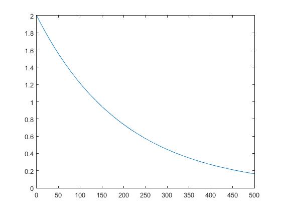
>> plot(t,ca,t,cb)
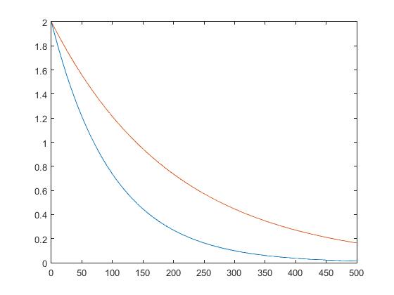
ca will have the lowest output
sooner.
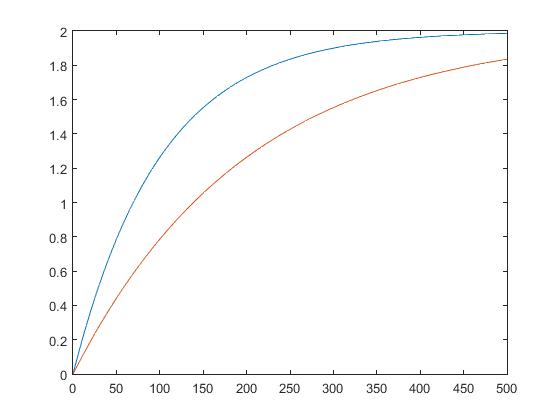
>> ca2=2*(1-exp(-t/100));
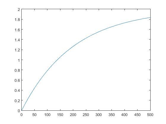
>> cb2=2*(1-exp(-t/200));
>> plot(t,ca2,t,cb2)
>> plot(t,ca2)

>> plot(t,cb2)
2, Assignment 2

t=linspace(0,4*pi);
>> theo=7.29*sin(2*t+0.727);
>>
mat=3*sin(2*t+10*pi/180)+5*cos(2*t-30*pi/180);
>> plot(t,theo,t,mat);

>>
mat1=3*sin(2*t+10*pi/180);
>>
mat2=5*cos(2*t-30*pi/180);
>>
plot(t,theo,t,mat,t,mat1,t,mat2)

2.
f=10;
>> w=2*pi*f;
>> theo=7.29*sin(w*t+0.727);
>>
mat=3*sin(w*t+10*pi/180)+5*cos(w*t-30*pi/180);
>> plot(t,theo,t,mat);

A Script to implement this with
any f(HZ)
>> w=2*pi*f;
>> theo=7.29*sin(w*t+0.727);
>>
mat=3*sin(w*t+10*pi/180)+5*cos(w*t-30*pi/180);
>> plot(t,theo,t,mat);
f=20;

COMPLEX NUMBER
OPERATIONS WITH COMPLEX NUMBERS
>> A=2+2j, B=-1+3j, C=2+j
A =
2.0000 + 2.0000i
B =
-1.0000 + 3.0000i
C =
2.0000 + 1.0000i
>> D=(A*B)/C
D =
-2.4000 + 3.2000i
>> E=(A+B)*C
E =
-3.0000 +11.0000i
FUNCTIONS TO CONVERT FROM RECTANGULAR TO POLAR
EXERCISE 1:
>> A=3+4j; B=3-2j;
C=2*exp(50*pi/180*j);
>> D=(A+C)/B
D =
0.1379 + 1.9360i
EXERCISE 2:
>> E
E =
-3.0000 +11.0000i
>> abs(E)
ans =
11.4018
>> angle(E)
ans =
1.8370
>> angle(E)*180/pi
ans =
105.2551
ASSIGNMENT
>> A1=3+2j; A2=-1+4j; B=2-2j
B =
2.0000 - 2.0000i
>> A1=3+2j; A2=-1+4j;
B=2-2j;
>> C=(A1*B)/A2
C =
-1.0588 - 2.2353i

2.
>> angle(A1)*180/pi, abs(A1)
ans =
33.6901
ans =
3.6056
>> %3.6056<33.6901
>> angle(A2)*180/pi, abs(A2)
ans =
104.0362
ans =
4.1231
>>%4.1<104
>> 4<104
ans =
1
>> angle(B)*180/pi, abs(B)
ans =
-45
ans =
2.8284
>> %2.8<-45
3.
>> D=(A1+B)*A2
D =
-5.0000 +20.0000i
4.
>> T=[8+8j 2j;2j 4-4j]
>> P=[50j;-30j]
>> I=inv(T)*P
I =
2.0588 + 2.9412i
5.0000 - 3.5294i
>> I2=5-3.5294j;
angle(I2)*180/pi, abs(I2)
ans =
-35.2175
ans =
6.1202
SOLVING FOR ROOTS OF EQUATIONS
EXERCISE 1
>> p=[1 4 3];
>> r=roots(p)
r =
-3
-1
Assignment
1. >> p1=[1 1 4];
>> p2=[1 3 0 3];
>> p3=[1 3 4 2 7];
>> r1=roots(p1)
r1 =
-0.5000 + 1.9365i
-0.5000 - 1.9365i
>> r2=roots(p2)
r2 =
-3.2790 + 0.0000i
0.1395 + 0.9463i
0.1395 - 0.9463i
>> r3=roots(p3)
r3 =
-1.8222 + 1.2680i
-1.8222 - 1.2680i
0.3222 + 1.1474i
0.3222 - 1.1474i
2.
>> p=[1 5 7 3];
>> s=roots(p)
s =
-3.0000 + 0.0000i
-1.0000 + 0.0000i
-1.0000 - 0.0000i

>> T=[1 1 0;2 4 1;1 3 3];
>> I=[0;1;7];
>> K=inv(T)*I
K =
1
-1
3
>> p=[1 5 7 3];
>> s=roots(p)
s =
-3.0000 + 0.0000i
-1.0000 + 0.0000i
-1.0000 - 0.0000i

>> T=[1 1 0;2 4 1;1 3 3];
>> I=[0;1;7];
>> K=inv(T)*I
K =
1
-1
3
No comments:
Post a Comment